 Works on My GPU
First post in the ML & AI section, and a deliberate first choice: this blog's GPU section has spent several posts making one specific computation faster, without ever explaining what that computation actually is. This post is that missing piece: the Transformer architecture, from "Attention Is All You Need" (Vaswani et al., 2017).
The problem it replaced
Before Transformers, sequence models were built on recurrence — an RNN processes a sequence one token at a time, each step depending on the previous one's hidden state. That has two real costs: it's inherently sequential (you can't compute step 10 before step 9 finishes, which means no parallelizing across the sequence during training), and information from early tokens has to survive being passed through many sequential updates to still matter later, which in practice it often doesn't.
The Transformer's core move is to drop recurrence entirely and let every position look directly at every other position, all at once, through self-attention.
Scaled dot-product attention
The whole mechanism is one formula:
Attention(Q, K, V) = softmax(QKᵀ / √d_k) V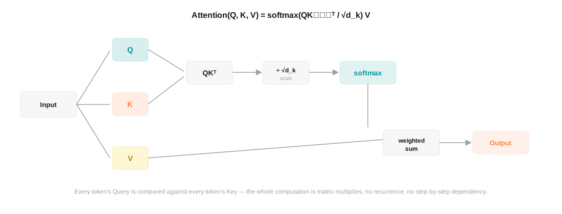
Each token's embedding gets projected (via learned linear layers) into three vectors: a Query (what this token is looking for), a Key (what this token offers to be matched against), and a Value (what this token actually contributes if attended to). The steps:
QKᵀ— every Query is dotted against every Key, producing a score for how much each token should attend to every other token./ √d_k— the scores are divided by the square root of the key dimension. Without this, large dot products (which get larger asd_kgrows) push the softmax into regions with extremely small gradients, making training unstable.softmax— turns the scores for each token into a probability distribution over all other tokens: the attention weights.× V— the output is a weighted sum of every token's Value vector, weighted by those attention weights.
This is why the whole thing maps so cleanly onto a GPU: there's no
step that depends on the previous step finishing. QKᵀ is a matrix
multiply over the entire sequence at once — exactly the kind of
operation the CUTLASS and
WGMMA posts in the GPU section are
about accelerating.
Multi-head attention
The original paper doesn't run one attention computation — it runs
8 in parallel ("heads"), each with its own learned Q/K/V
projections into a smaller dimension: d_model = 512, split across
h = 8 heads, giving each head d_k = d_v = 512/8 = 64. Each head's
output is concatenated back together and passed through one more
linear projection.
The point of splitting instead of using one larger attention computation: different heads consistently end up specializing in different kinds of relationships (e.g. one attending mostly to the previous token, another tracking longer-range syntactic dependencies) — splitting gives the model room to represent several different "types" of attention simultaneously, rather than averaging them into one.
Positional encoding
Attention has no built-in sense of order — QKᵀ treats the sequence
as an unordered set of tokens unless something tells it otherwise. The
original paper injects position information directly into the input
embeddings using fixed sinusoidal functions:
PE(pos, 2i)   = sin(pos / 10000^(2i / d_model))
PE(pos, 2i+1) = cos(pos / 10000^(2i / d_model))
Each embedding dimension corresponds to a sinusoid at a different frequency; added to the token embedding, this gives the model a signal for relative position that generalizes to sequence lengths it wasn't trained on. (Most modern LLMs have since moved to other schemes like RoPE, but the original sinusoidal version is what established that position needs to be injected explicitly at all.)
The full block
Attention alone isn't the whole layer. Each Transformer layer wraps
both the attention step and a position-wise feed-forward network
(two linear layers with a ReLU between them, expanding to
d_ff = 2048 and back down to d_model = 512) in a residual
connection followed by layer normalization:
output = LayerNorm(x + Sublayer(x))applied around both the attention sub-layer and the feed-forward
sub-layer. The original architecture stacks N = 6 of these layers in
both an encoder and a decoder (the decoder additionally attends to the
encoder's output) — trained on WMT 2014 English-to-German translation,
this setup reached 28.4 BLEU, beating every prior architecture on that
benchmark while training faster.
What changed since 2017
Most LLMs today don't use the original encoder-decoder shape — GPT-style
models kept only the decoder stack (self-attention restricted to only
look at earlier positions, since generation happens left to right) and
dropped the encoder entirely. The core mechanism — scaled dot-product
attention, multi-head splitting, residual + layer norm blocks — is
unchanged; what's evolved since is mostly around it: positional
schemes, normalization placement, and, as covered in this blog's GPU
section, exactly how that QKᵀ and the softmax get executed on real
hardware. FlashAttention is a
different way to compute the same formula on this page without
materializing the full attention matrix;
PagedAttention is about how the K and V
vectors get stored and reused once the model is actually serving
requests. Same formula, entirely different engineering problem once
you're running it at scale.
References
Attention flow diagram above is original artwork made for this post.